Overview

TimechoDB is an enterprise-grade time-series database developed by the core team behind Apache IoTDB.

In V2.0.8, we continue to strengthen the table model, enhance AI-native capabilities, and improve operational transparency and system robustness.

Key highlights include:

• OBJECT data type for large binary content

• Enhanced upgrade audit logging

• Optimized OPC UA support in the tree model

• Covariate forecasting and concurrent inference in AINode

• New system tables for observability

• Multiple security vulnerability fixes

For the complete release notes, please refer to: https://timecho.com/docs/UserGuide/latest/IoTDB-Introduction/Release-history_timecho.html

Key Updates in V2.0.8

Query Module

• Added a DataNode availability list, allowing users to inspect RPC addresses and ports of active nodes.

• Added a system table in the table model to track query execution latency statistics.

These improvements enhance cluster observability and operational transparency.

Storage Module

• Support for retrieving the full DDL(Data Definition Language) definition of tables and views via SQL.

• Optimized OPC UA protocol support in the tree model for improved interoperability in industrial IoT scenarios.

System Module

• Added OBJECT data type to the table model.

• Strengthened upgrade audit logging.

• Added a system table to monitor DataNode connection status.

AINode Enhancements

• Built-in chronos-2 model with covariate forecasting support.

• Built-in Timer-XL and Sundial models now support concurrent inference.

Stream Processing

• Creating a full synchronization pipe now automatically splits into:

  • a real-time pipe

  • a historical pipe

Remaining event counts can be inspected separately using Show pipes.

Security Fixes

This release addresses the following vulnerabilities:

• CVE-2025-12183

• CVE-2025-66566

• CVE-2025-11226

We strongly recommend upgrading to ensure system security.

Major Features: AINode Covariate Forecasting

Time-series forecasting in real-world systems rarely depends on a single variable. V2.0.8 introduces native covariate forecasting in AINode, enabling multivariate prediction with historical and future covariates.

• Univariate Forecasting: Predict a single target variable.

• Covariate Forecasting: Jointly predict multiple target variables while incorporating

  • Historical covariates

  • Future-known covariates

This improves predictive accuracy in complex industrial and business scenarios.

Syntax

SELECT * FROM FORECAST(
   model_ID,
   TARGETS, -- Get target covariates
   [HISTORY_COVS, -- String, get the historical covariates
   FUTURE_COVS, -- String, get future-known covariates
   OUTPUT_START_TIME,
   OUTPUT_LENGTH, 
   OUTPUT_INTERVAL,
   TIMECOL, 
   PRESERVE_INPUT,
   model_OPTIONS]?
)

Parameter Description

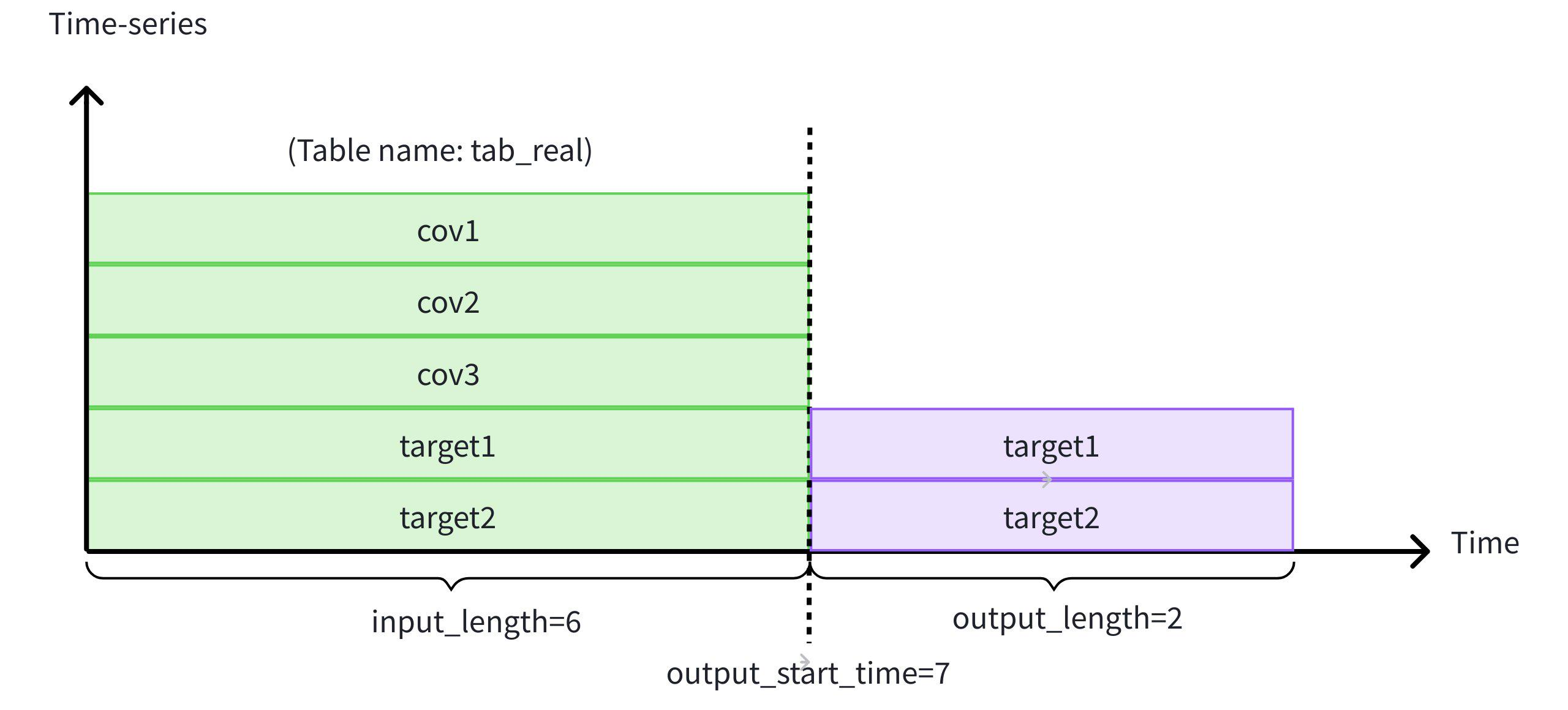
Example 1: Forecast with Historical Covariates

Create a database and table source, insert the test data:

-- 1. Create database
CREATE DATABASE testdb;
USE testdb;

-- 2. Create table source
create table tab_real (
    target1 DOUBLE FIELD, 
    target2 DOUBLE FIELD, 
    cov1 DOUBLE FIELD, 
    cov2 DOUBLE FIELD, 
    cov3 DOUBLE FIELD
);

-- 3. Insert test data
INSERT INTO tab_real (time, target1, target2, cov1, cov2, cov3) VALUES
(1, 1.0, 1.0, 1.0, 1.0, 1.0),
(2, 2.0, 2.0, 2.0, 2.0, 2.0),
(3, 3.0, 3.0, 3.0, 3.0, 3.0),
(4, 4.0, 4.0, 4.0, 4.0, 4.0),
(5, 5.0, 5.0, 5.0, 5.0, 5.0),
(6, 6.0, 6.0, 6.0, 6.0, 6.0),
(7, NULL, NULL, 7.0, NULL, NULL),
(8, NULL, NULL, 8.0, NULL, NULL);

Using the first 6 historical rows of target1, target2, and covariates cov1, cov2, cov3, we predict the next 2 timestamps, the result:

This content is only supported in a Feishu Docs

SELECT * FROM FORECAST (
    model_ID => 'chronos2',
    TARGETS => (
        SELECT TIME, target1, target2
        FROM etth.tab_real
        WHERE TIME < 7
        ORDER BY TIME DESC
        LIMIT 6) ORDER BY TIME,
    HISTORY_COVS => '
        SELECT TIME, cov1, cov2, cov3
        FROM etth.tab_real
        WHERE TIME < 7
        ORDER BY TIME DESC
        LIMIT 6',
    OUTPUT_LENGTH => 2
)

The excutation result:

+-----------------------------+-----------------+-----------------+
|                         time|          target1|          target2|
+-----------------------------+-----------------+-----------------+
|1970-01-01T08:00:00.007+08:00|7.338330268859863|7.338330268859863|
|1970-01-01T08:00:00.008+08:00| 8.02529525756836| 8.02529525756836|
+-----------------------------+-----------------+-----------------+
Total line number = 2
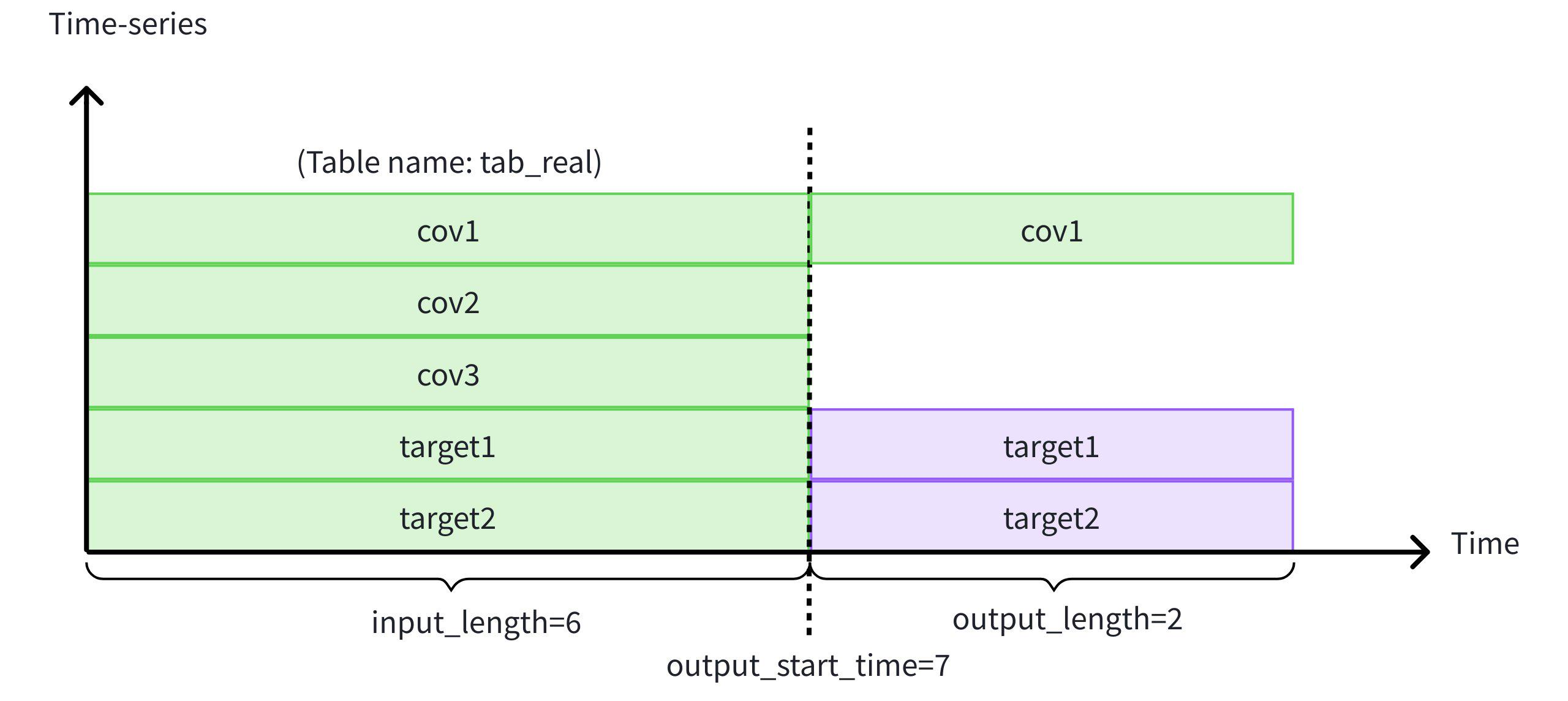
It costs 0.315s

Example 2: Forecast with Future-Known Covariates

In addition to historical covariates, we incorporate future-known cov1 values.

This content is only supported in a Feishu Docs

SELECT * FROM FORECAST (
    model_ID => 'chronos2',
    TARGETS => (
        SELECT TIME, target1, target2
        FROM etth.tab_real
        WHERE TIME < 7
        ORDER BY TIME DESC
        LIMIT 6
    ) ORDER BY TIME,
    HISTORY_COVS => '
        SELECT TIME, cov1, cov2, cov3
        FROM etth.tab_real
        WHERE TIME < 7
        ORDER BY TIME DESC
        LIMIT 6',
    FUTURE_COVS => '
        SELECT TIME, cov1
        FROM etth.tab_real
        WHERE TIME >= 7
        LIMIT 2',
    OUTPUT_LENGTH => 2
);

This enables hybrid forecasting scenarios common in demand planning, energy systems, and industrial control.

Major Features: OBJECT Data Type in Table model

Time-series systems increasingly require storage of unstructured binary assets (documents, audio, video, firmware, etc.) alongside structured telemetry.

V2.0.8 introduces the OBJECT data type to enable unified management within TimechoDB.

Key Characteristics

• Designed for large binary objects

• Physically stored under ${data_dir}/object_data

• Query results display metadata:

(Object) XX KB

• Raw content can be retrieved via READ_OBJECT()

Difference from BLOB

Current Limitations

In this release:

• Not supported in the tree model

• Not yet compatible with table model:

  • Data synchronization

  • Import/export

  • Data backfill

These will be supported in future versions.

Writing OBJECT Data

Syntax

INSERT INTO tableName(time, columnName)
VALUES(timeValue, to_object(isEOF, offset, content));

Parameters

Example: Segmented Write

Add an OBJECT-type column s1 to table table1, and write an OBJECT with a total size of 5 bytes.

ALTER TABLE table1 ADD COLUMN IF NOT EXISTS s1 OBJECT FIELD COMMENT 'objecttype'

• Non-segmented write

insert into table1(time, device_id, s1) values(now(), 'tag1', to_object(true, 0, X'696F746462'));

• Segmented write

--First write：to_object(false, 0, X'696F')
insert into table1(time, device_id, s1) values(1, 'tag1', to_object(false, 0, X'696F'));
--Second write：to_object(false, 2, X'7464')
insert into table1(time, device_id, s1) values(1, 'tag1', to_object(false, 2, X'7464'));
--Third write：to_object(true, 4, X'62')
insert into table1(time, device_id, s1) values(1, 'tag1', to_object(true, 4, X'62'));

Querying Data

Notes:

• The OBJECT type does not support the GROUP BY, ORDER BY, OFFSET, or LIMIT clauses.

• When used with the FILL clause, only the PREVIOUS fill policy is supported.

Example 1: Querying OBJECT Data Directly

select s1 from table1 where device_id = 'tag1'

Execution result:

+------------+
|          s1|
+------------+
|(Object) 5 B|
+------------+
Total line number = 1
It costs 0.428s

Example 2: Retrieving the Raw Content Using the READ_OBJECT Function

select read_object(s1) from table1 where device_id = 'tag1'

Execution result:

+------------+
|       _col0|
+------------+
|0x696f746462|
+------------+
Total line number = 1
It costs 0.188s

Conclusion

TimechoDB V2.0.8 strengthens the platform across below parts:

1. Data model extensibility (OBJECT)

2. AI-native forecasting capabilities

3. Operational visibility and security

By integrating advanced forecasting directly into SQL workflows and enabling unified management of structured and unstructured data, TimechoDB continues to evolve beyond a traditional time-series database into an intelligent data infrastructure platform.

For enterprise packages or technical consultation, please contact our team.

More in-depth technical analysis and live sessions will follow.

Stay tuned.